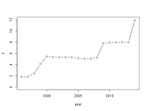
Figure 0. CER of UAH. 1 USD is exchanged for \( y \) UAH.
This is a paper for peer assessment for course “Introduction to Statistics for the Social Sciences” by Marco Steenbergen from University of Zurich.
Ukrainian currency (UAH) experienced several large drops (CER shocks) in its value within the last 20 years. Every drop in the value of a national currency automatically makes export more attractive and indirectly increases wages in exporting firms. According to economic theory, then workers migrate to exporting firms until wages are leveled out again. The goal of this research is to determine whether this adjustment of the job market to a CER shock is actually occurring.
First, I need to check that wages actually increase if export increases. The obvious model of this relationship is a linear equation \( Y=\alpha+\beta\cdot X \) where \( Y \) is the logarithm of the average wage and \( X \) is the logarithm of the amount of export per worker; the parameter \( \beta \) is a measure of dependency of wages on export. Export is considered an independent variable.
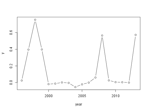
Second, I need to find out how this dependency develops with time. If the job market is adjusting, \( \beta \) should decrease to 0. Of course, further CER changes can disrupt this process of adjustment. Fortunately, 3 shocks in CER of UAH are separated by periods of stability as you can see on Figure 0 and Figure 1. (Data are obtained from: National Bank of Ukraine; page “Курси обміну валют”; link “Середній курс гривні до іноземних валют”/“Офіційний курс гривні до іноземних валют (середній за період)”; sheet “1996–2015”; row “100 доларів США”; unit: how much UAH is exchanged for 1e2 USD.)
Figure 0. CER of UAH. 1 USD is exchanged for \( y \) UAH.
Figure 1. Speed of change of CER of UAH. \( y=\operatorname{lb}(f(t+1)/f(t)) \) where \( f(t) \) is CER of UAH in year \( t \).
The idea is to measure the dependency at the beginning and the end of any period of stability. I will investigate the period from 2009 to 2013 because it's the only period I can obtain data for. Because it's improbable that the job market can completely adjust to a shock and make wages not dependent on export, I'd rather ask if \( \beta \) at the end of the period is less than a half of \( \beta \) at the beginning.
Because I cannot obtain data per firm, so I used data per region (oblast) of Ukraine. An experimental unit is a region. Amount of export, number of workers, and wages for every region are published by state agencies. Data source for export, number of workers, and the average wage is State Statistics Service of Ukraine. The leftmost column in all tables contains a region of Ukraine. A data source for wages: page “Динаміка середньомісячної заробітної плати по регіонах у 1995-2014 роках”; unit: UAH per month. Other sources are described in Table 0.
Table 0. Data sources.
| type of data | the beginning of the period | the end of the period |
| export | page
“Обсяги експорту-імпорту товарів за регіонами України за
2009 року” column “Експорт”/“млн. дол. США” unit: 1e6 USD per year |
page
“Обсяги експорту-імпорту товарів за регіонами України за
2013 рік” column “Експорт”/“тис. дол. США” unit: 1e3 USD per year |
| number of workers | page link “Статистичний збірник «Регіони України»”/“2012 рік”/“Частина I” file “1_04(2013).doc” Table 4.2. “Зайняте населення у віці 15–70 років” (“Employed aged 15–70”) column “2009”/“тис. осіб” unit: 1e3 person |
page link “Статистичний збірник «Регіони України»”/“2013 рік”/“Частина I” file “1_04(2014).doc” Table 4.2. “Зайняте населення у віці 15–70 років” (“Employed aged 15–70”) column “2013”/“тис. осіб” unit: 1e3 person |
| combined | link | link |
I combined the data, converted units of measurement, and saved it into files in CSV format; links are in Table 0. Meaning of data fields is described in Table 1.
Table 1. Meaning of fields in combined data files.
| field | meaning | unit |
|---|---|---|
| wage | the average wage per worker | USD per year |
| worker | the number of workers in the region | person |
| export | the export of the region | USD per year |
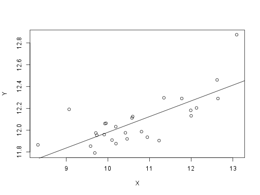
I've chosen a significance level of 0.01. The number of units \( n \) is 27. I define variables \( X=\operatorname{lb}(\mathrm{export}/\mathrm{worker}) \) and \( Y=\operatorname{lb}(\mathrm{wage}) \) on the fields of the combined data files. The data are depicted in Figure 2 and Figure 3.
Figure 2. The dependency of wages on export at the beginning of the period. See explanations for \( X \) and \( Y \) in the text.
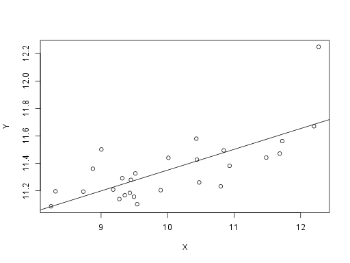
Figure 3. The dependency of wages on export at the end of the period. See explanations for \( X \) and \( Y \) in the text.
The dependency of \( Y \) on \( X \) is assumed to be \( Y=\alpha+\beta\cdot X \). I'm only interested in an estimate of \( \beta \). Computed statistics, hypotheses, and conclusions are in Table 2. For the beginning of the period, the alternative hypothesis is that \( Y \) increases if \( X \) increases. For the end of the period, the alternative hypothesis is that the job market compensated at least a half of initial dependency, i. e. \( \beta_0 \) of the end of the period is a half of \( b \) of the beginning of the period. The test statistic \( t \) is computed as \( (b-\beta_0)/s_b \) (where \( s_b = \sqrt{s_Y^2/s_X^2-b^2 \over n-2}) \) and is distributed as \( \mathcal{T}(n-2) \).
Table 2. Results.
| value | the beginning of the period | the end of the period |
|---|---|---|
| arithmetic mean of \( X \), \( \overline X \) | 10.03468 | 10.70512 |
| variance of \( X \), \( s_X^2 \) | 1.307696 | 1.376685 |
| standard deviation of \( X \), \( s_X \) | 1.1435453642072972 | 1.1733222063866344 |
| arithmetic mean of \( Y \), \( \overline Y \) | 11.35582 | 12.08186 |
| variance of \( Y \), \( s_Y^2 \) | 0.05704802 | 0.0520311 |
| standard deviation of \( Y \), \( s_Y \) | 0.23884727337778006 | 0.22810326608797166 |
| covariance, \( s_{XY} \) | 0.19809 | 0.1986018 |
| Pearson's correlation coefficient, \( r \) | 0.7252518853987138 | 0.7420520792980562 |
| slope of the best fit line, \( b \) | 0.15148016052660557 | 0.1442608875668726 |
| \( \beta_0 \) | 0 | 0.07574008026330278 |
| null hypothesis, \( H_0 \) | \( \beta \leq \beta_0 \) | \( \beta \geq \beta_0 \) |
| alternative hypothesis, \( H_A \) | \( \beta > \beta_0 \) | \( \beta < \beta_0 \) |
| \( s_b \) | 0.028760107274780566 | 0.026063983498690324 |
| test statistic, \( t \) | 5.267023487754405 | 2.6289460821294983 |
| rejection region for \( t \) | \( t \geq 2.485107 \) | \( t \leq -2.485107 \) |
| rejection region for \( \beta_0 \) | \( \beta_0 \leq 0.08000821661729746 \) | \( \beta_0 \geq 0.20903267540735243 \) |
| \( H_0 \) is rejected | yes | no |
Exporting firms are attractive to employees in Ukraine because they offer greater wages. According to data for year 2013, wages rise by 10.5164 % if the export per worker rises 2 times, and the export per worker varies by 27 times across regions. This dependency has r=0.7420521. The job market can't adjust to this inequality after 4 years; the dependency of wages on export remains practically the same. This can be explained by a barrier that precludes workers from entering exporting firms.